During my telecommunications degree I took a course on signals and noise, I spent a lot of evenings writing probability by hand: expectations, variances, the odds of two random variables landing in some region. It always sucked, when I tried to run it on a computer, so much boilerplate.
That wish became NoiseLang. I started it about nine years ago, however, I never finished it. Only recently, I brought it back thanks to AI tools and something far more ambitious than what I could have built alone the first time.
Everything is a distribution
The whole language hangs on one idea, that every value is a probability distribution. A plain number is a Dirac spike, a distribution with all its weight on a single value. Since constants and random variables are the same kind of object, every operator in the language maps distributions to distributions.
Purists will tell you that the Dirac delta belongs to continuous densities and has no business on a
six-sided die, and they are right. What I mean is the Dirac measure, all the weight on one point,
which works fine on a die. Noise never evaluates a density anyway, it draws samples. And a constant
collapses back to a plain integer in the graph, so 5 costs nothing.
A name always refers to one fixed node, the same way X is the same X across a whole page of math.
So X + X is 2X and X - X is exactly 0. If you want variable independence you
write separate draws, ie, using ~ multiple times, or ~[N] to draw N independent variables into a vector.
X ~ unif_int(1, 6)
Y ~ unif_int(1, 6)
X + Y                 # two independent dice, a real 2d6 distribution
Nothing runs until you ask for some results, for example, P(X + Y < 10), at that moment it forces the runtime to
run millions of simulations (across all cores, if available) and return an estimate with a standard error attached.
Bday = unif_int(1, 365)
days ~[23] Bday          # 23 people in a room
P(has_duplicates(days))  # the birthday paradox, about 0.507
This is much easier to watch than to describe, so I built some cool demos!
Every value is a distribution
A = 5D1 ~ unif_int(1, 6)D2 ~ unif_int(1, 6)S = A + D1 + D2E(S)A number is a distribution
A = 5 looks like a plain constant, and it is, but Noise
sees it as a probability distribution where every draw lands on 5. Statisticians call this a
Dirac delta, a single infinitely-thin spike.
The tilde spreads it out
D1 ~ unif_int(1, 6) binds a fair die, a discrete
uniform where all six faces are equally likely. The spike fans out into six flat bars, so
D1 is now uncertain, but you still write it like
any other variable.
Join them and a bell appears
Add the constant and two independent dice with S = A + D1 +
D2. The flat shapes convolve into a triangle peaked at 12, already curving
toward a bell, and if you join a few more they sharpen into a true Gaussian. That's the
central limit theorem showing up for free!
A query collapses millions of draws
Nothing runs until you ask. E(S), the expected
value, fires a Monte Carlo pass that averages millions of rolls into one number, and by
the law of large numbers the running mean settles on 12. You
wrote a few lines of math, and an expert-level kernel ran underneath.
Why it sat for nine years
The design was never the hard part, because a parser and a tree-walking interpreter for this language is a weekend of work. The problem was everything else, writing an efficient Monte Carlo runtime, instead of a naive interpreter, conditional bayesian inference, and more.
Current version is a compiler with a GPU backend (WGSL through wgpu), a WASM backend, and a pile of careful numerical code, so for a cute-weekend project it stayed permanently out of reach.
Building the ambitious version with an agent
At my day job and side projects, I am experimenting with the boundaries of what today’s AI agents can do. For example, I am also porting a game I built 15 years ago for iOS, in archaic Objective-C to a modern game engine (with relative success).
With NoiseLang, I realized, AI is great at building the JIT parts, the runtime parts, the numerical parts, but it sucks at coming up with good language design ideas, many times overriding existing language features for different purposes, or coming up with different syntax for non-orthogonal features.
One IR, three backends
The first plan was to compile the graph into WASM and let a WASM runtime JIT it for me, because that runtime was surely going to optimize better than any compiler I could write myself. While exploring that, I realized I could reach for the JIT optimizer directly and skip the WASM step, so the first native backend was a Cranelift JIT, a killer library for a project like this, NoiseLang ran at native speed and I barely wrote any compiler. That JIT is gone now. Keep reading, because the reason it left is my favorite part of the whole project.
~ and the distribution constructors build an append-only DAG called the RvGraph. This graph is the single source of truth,
which is later converted into three different code paths:
- a columnar batch interpreter that works everywhere and acts as the correctness oracle;
- a WGSL emitter that fuses a whole expression into one GPU compute shader;
- a WASM emitter that does the same fused kernel for the browser’s CPU.
One shared module defines what the graph means, so the two code generators stay thin and cannot drift apart. Anything a backend can’t successfully compile falls back to the interpreter, and the results stay identical across backends and core counts. All tests run in all three code paths and compared to be bit-identical.
The engine picks the path per query, the same way a SQL query planner picks an execution plan: a
cost model keeps the small queries on the vectorized interpreter, fans the medium ones out across
every core with a work-stealing reducer, and sends the heavy ones to the GPU as one fused compute
shader. You write P(...), the planner does the rest.
Making the Monte Carlo loop cheap
All the performance work is about one loop: draw a few million samples, evaluate the expression on each, and reduce the results. A handful of techniques carry most of it, while keeping the results deterministic (that was the hard part).
Kernel fusion keeps every intermediate value in registers, so an arithmetic-heavy expression stays in registers. The PRNG compiles into the
kernel, and the ln, sin, and cos become inline polynomial
approximations, speeding up the kernel by a factor of 2.
My favorite trick used to be in the RNG. The original generator (xoshiro256++) is a serial dependency chain, so instead of fighting that, the kernel ran four independent streams at once and let the out-of-order core overlap them. That trick is retired now, and the reason is better than the trick: the RNG became counter-based (squares64), a middle-square hash where every draw is a pure function of (seed, lane, source). No state to thread through the loop means any slice of the sample space can run on any core, or any GPU thread, and land bit-identical. And it is not a random pick (pun intended), the exact bit stream the engine consumes passed 1 TB of PractRand with zero anomalies.
On my 14-core M4 Pro, a one-line P(...) sustains around 5.8 billion samples per second and scales
about 9.6× from one core to all of them. Per core, the JIT kernel ran within about 1.15× of
hand-written Rust compiled by LLVM, which told me the CPU codegen had hit its ceiling. The same
fused loop, emitted as WASM, runs at roughly half to three-quarters of native speed inside V8.
Estimating π with Monte Carlo
play in the playground ↗X ~ rand::unif(-1, 1)Y ~ rand::unif(-1, 1) C = X^2 + Y^2 < 1 4 * P(C)Two random draws
This is the same ~ as before, used twice.
X ~ unif(-1, 1) and Y ~ unif(-1,
1) each draw a number anywhere in [-1, 1], and together they pick a random point in
the square.
Ask one yes/no question
C = X² + Y² < 1 is true exactly when the point falls
inside the unit circle. In Noise that comparison is itself a random variable, a Bernoulli
that lands true or false on each draw.
Now throw the darts
Each dart is one draw of (X, Y), teal when it lands inside
the circle and grey when it doesn't. They scatter evenly, because the uniform draws don't
favor any point over another.
Four times the fraction is π
The circle covers π/4 of the square's area, so the teal share hovers around π/4, and that
makes 4 * P(C) an estimate of π. The more darts you throw,
the sharper the estimate gets.
The GPU ate the JIT
A few weeks after I published this article, I deleted the JIT. The idea clicked when I noticed that a Monte Carlo query is already shaped like a compute shader: one pure kernel evaluated over millions of independent lanes, then a reduce to fold them down. That is exactly the GPU compute model, so the RvGraph got a WGSL lowering, and thanks to wgpu the same emitter reaches Metal, Vulkan and DirectX 12 on native, and WebGPU in the browser. One GPU backend to maintain, instead of one per platform.
Then I measured the full example corpus on the M4 Pro:
| backend | corpus total | speedup |
|---|---|---|
| interpreter | 3854 ms | 1.00× |
| Cranelift JIT | 3274 ms | 1.18× |
| GPU | 923 ms | 4.17× |
| JIT + GPU | 843 ms | 4.57× |
Once the GPU exists, everything the JIT adds is 80 ms, and it only ever worked on native. So it went, 1,834 lines and four dependencies deleted, and the shipped CLI jumped from the interpreter to the GPU by default. Deleting a backend was the fastest release I ever cut!
The heavy examples are where it gets fun. A quantization example that draws random rotation matrices
went from 1474 ms to 55 ms (26×). The 100-prisoners simulation needed real compiler work first:
by the time the emitter sees the graph, a for loop is unrolled into ~15,000 data-dependent
reads, and the Metal shader compiler takes 2.2 seconds to chew on that. The fix was to capture the
loop as a single node at eval time and emit it back as an actual WGSL loop, and the simulation
dropped from 59 ms to 2.8 ms.
Where Noise sits
NoiseLang is a toy language, you probably should not use it for anything serious, however I wish this language existed during my university days.
For a language nerd, it’s a small expression-based language over a static random-variable algebra, with forward Monte Carlo and rejection-based conditioning.
You might ask, how does it compare to NumPy or Stan? NumPy makes you write the simulation yourself, and Stan makes you declare a model and wait for a sampler. Noise lets you write the probability as math while running Monte Carlo under the hood to get the answer.
| Noise | NumPy | Stan | PyMC | |
|---|---|---|---|---|
| What it is | RV algebra + Monte Carlo | array numerics | declarative Bayesian modeling | Bayesian modeling in Python |
| Core abstraction | every value is a distribution | n-d arrays | data / parameters / model blocks | with Model() context |
| Getting an answer | P / E / Var / Q force sampling | you write the loop | compile → NUTS → summarize | pm.sample() → arviz |
| Inference | forward MC + rejection conditioning | none (you build it) | HMC / NUTS at scale | HMC / NUTS, VI, SMC |
| Setup to first answer | zero — type in a browser | import numpy | install toolchain, compile | install stack, build a context |
| Visualization | built into the language | matplotlib (separate) | bayesplot (external) | arviz (separate) |
| Runs in the browser | yes — WASM, no install | no | no | no |
Stan and PyMC beat Noise at the thing they’re built for, fitting a posterior to lots of continuous data with their HMC/NUTS samplers, and NumPy beats it at raw array crunching. Conditioning in Noise is rejection-based, so it works great for a handful of discrete observations but becomes useless for ten thousand continuous measurements, and there is no stateful simulation yet (no Markov chains yet). Noise wins when you have a probability question and you wanna know the answer without much hassle.
So use Noise for the whiteboard stage of a problem, when you want to run the math you just wrote, and move to Stan or PyMC when you need a real posterior, or to NumPy and JAX when you need to go to production.
Back to signals and noise
Going back to my university days, there was this subject called “Señales Aleatorias Y Ruido”, which is a spanish translation of “Random Signals and Noise”.
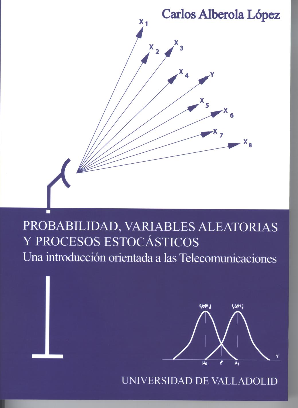
The textbook, in all its glory.
This subject was the nightmare of many students, including myself, in fact, I failed it. Truth be told, I didn’t put enough effort into it during the first year, but it changed when I had the take the same subject again in the second year. The professor was great, and made the subject interesting. The things that blew my mind was how he could model why FM survives a noisy channel when AM doesn’t.
So, here is my tribute to the subject, a one-screen Noise program that models why FM survives a noisy channel when AM doesn’t.
AM vs FM
play in the playground ↗msg = 0.3 * signal::sine(3); am_modulate(m) = 1 + m;fm_modulate(m, swing) = exp(i * swing * m); static ~ signal::noise_white_complex(0.4);rx_am = am_modulate(msg) + static;rx_fm = fm_modulate(msg, 3) + static; am_demodulate(c) = abs(c) - 1;fm_demodulate(c, swing) = arg(c) / swing;rec_am = am_demodulate(rx_am);rec_fm = fm_demodulate(rx_fm, 3); Print("AM error", E(mse(rec_am, msg)));Print("FM error", E(mse(rec_fm, msg)));scroll through the steps →
The message
In Noise a value can carry a whole signal, and here it's a gentle tone, a slow three-cycle sine. This is what we want to send through a noisy channel and get back intact.
AM puts the message in the length
The carrier is a complex number, a spinning arrow. AM's modulator puts the message in the arrow's length, so the tip slides in and out, crossing the unit circle as the message rises and falls.
FM puts it in the angle
FM puts the same message in the angle instead, so the tip rides along the unit circle while its length stays fixed. The information is identical, just encoded in rotation.
Add the same static
Now identical white noise hits both tips. It smears AM along exactly the radius it reads from, but it only nudges FM around the circle, barely changing the angle. You can see it in the shape of the two clouds.
Recover
Demodulate: read the length back for AM and the angle back for FM, laid over the original message. You can already see it, the AM trace comes back ragged while the FM one hugs the original.
Same storm, very different damage
mse averages the error over the waveform, and
E averages that over many draws of the static. Same signal
energy, same noise energy, yet FM comes back about 5× cleaner, and in the small-noise limit
the advantage approaches swing² = 9. That is the bandwidth it spent on the angle paying
off.
One caveat, and roger_ on Hacker News caught it before I did. The program above modulates phase, not
frequency, so technically it is PM. For the single tone I am sending, PM and FM are the same thing up
to a scale factor and a shift, so the demo still shows what I want it to show, but real FM would
differentiate the message before it goes into the phase. Now I want to write that version, because FM
should pull even further ahead once the message stops being a single tone.
Run NoiseLang in the browser
Everything above runs on @noiselang/core, thanks to the Rust engine compiled to WebAssembly.
npm install @noiselang/coreimport { run } from "@noiselang/core";
const result = await run(`
X ~ rand::unif(-1, 1);
Y ~ rand::unif(-1, 1);
4 * P(X^2 + Y^2 < 1)
`);
console.log(result.value); // "3.1415…" — the last statement's value
console.log(result.output); // everything Print(...) emittedrun never throws, failures come back on result.error with a source span. There is also
runWithIntrospection, the API behind the variable inspector at noiselang.com.
And when the page has WebGPU available, the heavy queries run on your GPU with the same WGSL shaders as native. Everything else stays on the WASM kernel, so nothing breaks on browsers that don’t have it.
NoiseLang is playable in the browser at noiselang.com. Open it, type
X ~ unif(-1, 1); Y ~ unif(-1, 1); 4 * P(X^2 + Y^2 < 1), and watch a few million
draws estimate π from your browser tab.
Appendix: prior art
I posted this on Hacker News and the thread turned into a reading list, which is the best thing that can happen to you when you ship a toy language. NoiseLang is not the first language to treat probability as a first-class value, not even close, so here is what people pointed me to:
- monad-bayes, a Haskell library where the same “everything is a distribution” idea falls out of the monad, courtesy of
bradrn. I had no idea Haskell could express this so directly. - webppl, Anglican, Stan and PyMC, the real probabilistic programming languages, suggested by
chrisra. If you have an actual model to fit, go there, not here. - diceplots.com by
qdotme, which keeps the distributions exactly analytical at every step and never samples. The opposite trade-off to mine, and a fun one. - “General Purpose Convolution Algorithm in S4-Classes by means of FFT” by Ruckdeschel and Kohl, sent by
data-ottawa. It is the paper behind the R packagedistr, and it overloads+,-,*,/on distributions by computing the convolutions with an FFT instead of sampling them. Exactly the operator algebra I wanted, arrived at from the other direction. kccqzy’s work on probabilistic program inference, which handles loops without Monte Carlo at all. He also asked the question I was hoping nobody would ask, which is how NoiseLang handles loops, and the answer is that it does not.
Big thanks also to RossBencina and thrtythreeforty, who pushed on the RNG trick until I understood
my own benchmark better, and to roger_, who noticed that my FM demo is really doing phase modulation.
This is why you post your toys!